Deep learning enhanced reduced order models

Major Activities

Deep Learning Enhanced Reduced Order Models

Inverse problems are pervasive mathematical methods in inferring knowledge from observational and experimental data by leveraging simulations and models. Unlike direct inference methods, inverse problem approaches typically require many forward model solves usually governed by partial differential equations. This a crucial bottleneck in determining the feasibility of such methods. Reduced-Order Models accurately capture supposedly important physics of the forward model in the reduced subspaces in a computationally efficient manner, thereby accelerating the inverse problem solution at the cost of accuracy. We presented a data-driven technique to augment the accuracy of reduced order models by learning their error compared to high-fidelity models and experimental data with the goal of accelerating many-query problems in deterministic inverse problems. We presented preliminary results that support our approach in accelerating parameter-to-observable maps to solve inverse problems in steady heat conduction problems, neutron transport equations, and advection-diffusion equations.

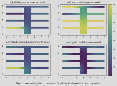
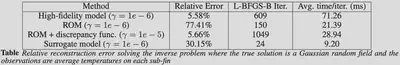
Validation of the proposed method is performed using numerical experiments. The inverse problem for steady heat conduction is posed as inferring conductivity parameters from sparse observations on a thermal fin. The finite element solution using a coarse mesh was considered as the high fidelity model. An affine decomposition of the resulting stiffness matrix along with projection of the governing equations to a reduced space was used to construct a reduced order model. The error was learned using a deep learning model in a data-driven fashion using simultaneous solves of the high fidelity model and the reduced model for training parameter values sampled from a Gaussian field. The relative error between the ground truth parameters and the parameters computed from solving inverse problems using the high fidelity model, the reduced order model, and the deep learning enhanced reduced order model is computed. The results show that the latter model shows comparable accuracy to the high fidelity model reconstructions while providing computational efficiency similar to that of the reduced order model.

The following form of the PDE-constrained optimization procedure is usually employed to obtain an estimate for the parameters by minimizing the objective function $$ J(\boldsymbol{w}, \mathbf{\kappa}) : \mathbb{R}^N \times \mathbb{R}^{N_u} \rightarrow \mathbb{R} $$ by solving \( \newcommand{\LRp}[1]{\left( #1 \right)} \)

$$\begin{eqnarray} \underset{\mathbf{\kappa}}{\min} \quad & J(\boldsymbol{w}, \mathbf{\kappa}) := \dfrac{1}{2} ||\mathbf{y}^{\text{obs}} - \mathbf{F}(\boldsymbol{w}(\mathbf{\kappa}))||_{\Sigma}^2 + \gamma \mathcal{R}(\mathbf{\kappa}) \ \text{s. t.} \quad & \mathbf{R}(\boldsymbol{w}, \mathbf{\kappa}) = 0 \end{eqnarray}$$

where $$\mathbf{y}^{\text{obs}}, \ \mathbf{F}, \ \kappa, \ \Sigma, \ \mathcal{R}(\mathbf{\kappa}), \ \gamma, \ \mathbb{R}$$ represents the measured observations, the parameter-to-observation map, parameter vector, measurement noise covariance, regularization operator introduced to make the inverse problem well-posed, coefficient of regularization, and the governing model respectively.

The proposed DL-enhanced ROM quantity of interest reads

$$\begin{equation} \mathbf{F}(\mathbf{\kappa}) = \tilde{\mathbf{y}}(\mathbf{\kappa}) = \mathbf{y}_r \LRp{\mathbf{\kappa}, \Phi} + \varepsilon_{\mathrm{NN}}(\mathbf{\kappa},\boldsymbol{\theta}) \end{equation}$$

where $$\Phi$$ is the reduced trial basis.

Model-Aware Deep Neural Networks

Training neural networks to accurately and efficiently solve physical problems purely using data-driven techniques require prohibitive amounts of data to be gathered from large number of experimentation scenarios. Mathematical models contain important information regarding the relationships between important quantities of interest. This information can be used to augment the training of neural networks. We formulated a neural network optimization framework that introduces the constraints posed by mathematical models as a penalization term to the neural network loss functions. This penalization term biases trained models towards minimizing the residuals of the constraint equations of the underlying mathematical model.

Deep learning optimization problems are usually solved using highly optimized tensor computation frameworks such as Tensorflow whereas mathematical models, particularly those that involve partial differential equations, are solved using various numerical libraries calibrated for physical quantities which may not be represented as tensors. The model-aware training of neural networks thus require interoperating these libraries by formulating physical models as tensor computations. We introduce the ability to encode physical constraints in linear elliptic problems defined using FEniCS, a library to solve partial differential equations, into Tensorflow’s neural network tensor-based loss functions. The combined loss function can be used to train model-aware neural networks with efficient consumption of observational data.

Furthermore, we formulated model-aware loss function to encode physical information for time-dependent problems by adding a term that penalizes errors between network predictions at a given time compared to the time-stepping prediction of the mathematical model. This introduces temporal dependencies in the quantities of interest to the neural network. Preliminary experiments in auto-encoding state in a time-dependent heat equation shows that the model-aware network shows better accuracy than a purely data-driven network.

Specific Objectives

Accelerating Inverse Problems using Reduced Order Models and Deep Learning

I am currently employing reduced order models improved by deep learning error models to accelerate solving inverse problems using aforementioned methods. The research paper will be submitted to the SIAM Journal on Scientific Computing. [2]

Preliminary Research on Stein-Variational Inference

I am currently exploring new research avenues on improving Bayesian inference using Stein-variational methods by incorporating reduced order models and model-aware deep learning.

Optimizing hyper-parameters of neural networks

Learning the error between the full model and the reduced model is a high-dimensional deep learning regression problem whose performance is sensitive to the particular architecture of the deep neural network model. These so-called hyperparameters of the deep learning model were determined using a Bayesian optimization framework. A Gaussian process surrogate model is employed to parametrize the performance of the neural network as a function of the hyper-parameters. This approach to pick hyper-parameters improves on grid search and random search as the sampling procedure better explores the hyper-parameter space by leveraging information from previous neural network architectures.

Spatial Averaging to Hyper-Reduce Model Order

The aforementioned deep learning error models for reduced order models enlarge the validity of projection-based model order reduction by capturing their errors in a data-driven fashion. In the regime of data prevalence, this corrective term can be used to learn errors for parameter dependent reduced order models created in a hyper-reduced fashion. Spatially-varying parameters governing the model can be averaged to induce an affine parameter dependence enabling precomputation of reduced order matrices, thereby accelerating evaluations of these models. This averaging process depends only on the geometry of the problem domain and can be performed cheaply using finite elements. The resulting computationally efficient ROMs can be improved in their accuracy using the deep learning error model in a data-driven fashion to create a hybrid model that is accurate and computationally efficient. This method was employed in solving inverse problems for steady heat conduction and advection-diffusion problems.

Significant Results

Accelerating Inverse Problems using Reduced Order Models and Deep Learning

The application of the enhanced reduced order model to neutron transport was verified using comparing the relative prediction error for a quantity of interest (scalar flux over a region of interest) compared to an expensive high-fidelity solution obtained from solving the full transport equations. The reduced order model for this problem is obtained in a physics-informed manner using a diffusion approximation to the collided component of the total transport flux along with energy group collapsing to form discrete energy bins from continuous energy. Further reduction in dimensionality is obtained using a projection of the the governing equations to a reduced space. The numerical experiment for this problem employed the iron-water benchmark, a standard 1-group 2D benchmark for transport solution techniques comprising of three spatial zones. The training parameter set for removal and scattering cross section values was randomly drawn uniformly from predetermined intervals. The neural network was trained to learn the discrepancy between the high-fidelity transport solution and the reduced order models. The average relative prediction error for the validation dataset shows comparable accuracy to the high-fidelity model when the deep learning correction was applied to the physics-informed reduced order models and the projection-based reduced order model. These experiments lend evidence to the ability of the discrepancy function to accurately model reduced order model errors compared to the high-fidelity transport solutions.

Bounding Deep Learning Error Models using Error Estimates

The errors committed by projection-based reduced order models in their predictions for quantities of interest can be rigorously bounded using the so-called dual-weighted residual method which requires an extra adjoint solution in a trial space finer than the space employed by the reduced order model. This estimate for the error in the quantity of interest can be computed during the online phase to produce bounds for the deep learning error model. The final activation function of the deep learning model is chosen to be the hyperbolic tangent multiplied point-wise with the estimate of the error, producing error model predictions within rigorous bounds. This method improves the deep learning error model training and prediction as verified by preliminary numerical experiments for advection-diffusion problems.

An estimate of the QoI error due to model order reduction can be obtained efficiently using the dual-weighted residual method [1]. To illustrate the a posteriori error estimation technique, we consider a system for a fixed parameter instance. The governing reduced order model is,

$$\begin{equation} \Psi^T \mathbf{R}(\Phi \boldsymbol{w}_r) = 0 \end{equation}$$

The error in the QoI can be approximated using a Taylor expansion

$$\begin{equation} \mathbf{y}(\boldsymbol{w}) - \mathbf{y}(\Phi \boldsymbol{w}_r) \approx \dfrac{\partial y}{\partial \boldsymbol{w}}(\Phi \boldsymbol{w}_r) (\boldsymbol{w} - \Phi \boldsymbol{w}_r) \end{equation}$$

The error in the residual due to the reduced model solution can also be approximated as,

$$\begin{equation} \mathbf{R}(\boldsymbol{w}) \approx \mathbf{R}(\Phi \boldsymbol{w}_r) + \dfrac{\partial \mathbf{R}}{\partial \boldsymbol{w}}(\phi \boldsymbol{w}_r) (\boldsymbol{w} - \Phi \boldsymbol{w}_r) = 0 \end{equation}$$

yielding,

$$\begin{equation} \boldsymbol{w} - \Phi \boldsymbol{w}_r \approx -\LRp{\dfrac{\partial \mathbf{R}}{\partial \boldsymbol{w}}(\phi \boldsymbol{w}_r)}^{-1}\mathbf{R}(\Phi \boldsymbol{w}_r) \end{equation}$$

Substituting the above equation in the QoI error yields,

$$\begin{equation} \mathbf{y}(\boldsymbol{w}) - \mathbf{y}(\Phi \boldsymbol{w}_r) \approx -\dfrac{\partial y}{\partial \boldsymbol{w}}(\Phi \boldsymbol{w}_r) \LRp{\dfrac{\partial \mathbf{R}}{\partial \boldsymbol{w}}(\phi \boldsymbol{w}_r)}^{-1}\mathbf{R}(\Phi \boldsymbol{w}_r) \end{equation}$$

where $$\lambda \in \mathrm{R}^d$$ is the solution to the adjoint equation

$$\begin{equation} \LRp{\dfrac{\partial \mathbf{R}}{\partial \boldsymbol{w}}(\phi \boldsymbol{w}_r)}^T \lambda = -\dfrac{\partial y}{\partial \boldsymbol{w}}(\Phi \boldsymbol{w}_r)^T \end{equation}$$

In order to avoid solving the adjoint equation in the high dimensional space, we approximate $$\tilde{\lambda}$$ using a trial space with basis $$\tilde{\Phi}$$ such that $$\tilde{\lambda} \approx \tilde{\Phi} \tilde{\lambda}_r$$ and solve the following reduced linear adjoint equation:

$$\begin{equation} \tilde{\Psi}^T \dfrac{\partial \mathbf{R}}{\partial \boldsymbol{w}}(\phi \boldsymbol{w}_r)^T \tilde{\Phi} \tilde{\lambda}_r = -\tilde{\Psi}^T \dfrac{\partial y}{\partial \boldsymbol{w}}(\Phi \boldsymbol{w}_r)^T \end{equation}$$

Thus, the estimate of the error in the QoI becomes $$\begin{equation} \mathbf{y}(\boldsymbol{w}) - \mathbf{y}(\Phi \boldsymbol{w}_r) \approx \tilde{\lambda}^T \mathbf{R}(\Phi \boldsymbol{w}_r) \end{equation}$$

yielding the a posteriori error bound

$$\begin{equation} |\mathbf{y}(\boldsymbol{w}) - \mathbf{y}(\Phi \boldsymbol{w}_r)| \le \sum_{i=1}^{d} |\tilde{\lambda}_i| |\mathbf{R}(\Phi \boldsymbol{w}_r)_i| \end{equation}$$

The trial and test reduced spaces for the adjoint solution is chosen to be finer than the reduced order model space by solving the latter system with a truncated basis obtained from the former system.

Uncertainty Quantification using MCMC

In order to quantify the uncertainty of the estimates provided by the inference using DL-enhanced reduced order models, a Bayesian formulation was developed. Markov Chain Monte Carlo methods provide the ability to draw samples from the posterior distribution of the parameter space conditioned on observational data while providing the ability to encode prior information. In order to efficiently explore the high-dimensional parameter spaces resulting from finite element discretizations of infinite-dimensional spaces, the Hamiltonian Monte Carlo algorithm is employed which leverages parameter sensitivity information to efficiently draw posterior samples. The No-U-Turn Sampler is used to set the path lengths in an adaptive fashion. The parameter sensitivities themselves are obtained using automatic differentiation for the deep learning components and the adjoint method for the reduced order model component. Despite using state-of-the-art Bayesian posterior sampling techniques, the required samples to accurately quantify uncertainty seem prohibitively expensive as seen from preliminary experiments. Future work aims to explore variational inference methods to improve the computational efficiency of the uncertainty quantification.

References

[1] Meyer, Marcus, and Hermann G. Matthies. “Efficient model reduction in non-linear dynamics using the Karhunen-Loeve expansion and dual-weighted-residual methods.” Computational Mechanics 31.1-2 (2003): 179-191.

[2] Sheriffdeen, Sheroze, et al. “Accelerating PDE-constrained Inverse Solutions with Deep Learning and Reduced Order Models.” arXiv preprint arXiv:1912.08864 (2019).